Introduction
Welcome to this book dedicated to Zero-Knowledge Proofs(ZK) and their applications in modern cryptography. Zero-Knowledge Proofs are magical, inspiring, passionate, and, more importantly, breathtaking. This book will compile documentation and specifications on ZK algorithms, aiming to provide researchers, developers, and cryptography enthusiasts with in-depth insights and guidance.
As this is a work in progress, we are continually learning and evolving our understanding of the subject. If you find any errors or areas for improvement, please feel free to provide feedback.
Please note that this book is a work in progress, and not necessarily to reflecting the latest developments in the ZK field.
Terminology
This document establishes a consistent terminology and notation for the concepts commonly used in the context of zero-knowledge proofs (ZKPs). It aims to make the presentation clear and concise, particularly for readers with a background in cryptography or mathematics. The following conventions will be used throughout the book:
Fields and Curves
- Finite Fields:
- : Denotes a general finite field of prime order .
- Elliptic Curves:
- : Scalar field
- : Base field
Algebra
In zero-knowledge proofs, algebra plays a crucial role as it provides the foundational framework for constructing complex mathematical structures and algorithms. These structures ensure the security and privacy of information, allowing verifiers to confirm the truth of a statement without revealing specific details. We will provide an introductory overview of groups, rings, fields, Number Theoretic Transform (NTT), and Multi-Scalar Multiplication (MSM).
Groups
Introduction
This document provides a simple introduction to group theory and its key role in cryptography. Group theory is essential for building many cryptographic systems, including encryption, digital signatures, and zero-knowledge proofs (ZKPs). These mathematical structures ensure that operations like encryption and authentication are secure and reliable.
We’ll start by defining groups, abelian groups, and cyclic groups, which are the backbone of many cryptographic algorithms. For example, the security of RSA encryption relies on group properties, and protocols like ECDSA use elliptic curves, which are based on group theory. Cyclic groups are crucial for creating secure ZKP systems like the Schnorr protocol, which is widely used for authentication.
Throughout the article, we’ll highlight how these abstract mathematical concepts directly contribute to secure communication in cryptography.
Groups And Abelian Groups
In cryptography, group theory plays a fundamental role, especially in modern public-key cryptography and protocol design. A group is an algebraic structure consisting of a set of elements and a binary operation that satisfies closure, associativity, identity element, and invertibility. Below are some key applications of group theory in cryptography:
- Underpins many widely used signature schemes, such as RSA and ECDSA.
- Many ZKP protocols use group operations, particularly cyclic groups, to construct secure proof systems. For instance, the Schnorr protocol is a zero-knowledge proof system based on cyclic groups and the discrete logarithm problem, widely used for authentication and privacy-preserving systems.
Let's begin with a definition and then some examples.
Basic Definitions
Binary operation: Let be a set. A binary operation is a map of sets: For ease of notation we write , for all in . Any binary operation on gives a way of combining elements. If (the set of integers , so denoted because the German word for numbers is Zahlen) then and are natural examples of binary operations.
Group: A group is a set , together with a binary operation , such that the following hold:
- (Associativity):The operation is associative;that is, for all in .
- (Existence of identity): There is an element (called the identity) in such that for all in .
- (Existence of inverses): For each element in , there is an element in (called an inverse of and denoted by ) such that .
- If is the of , then is the of .
- The group we have just defined may be represented by the symbol . This notation makes it explicit that the group consists of the and the .(Remember that, in general, there are other possible operations on , so it may not always be clear which is the group's operation unless we indicate it.) If there is no danger of confusion, we shall denote the group simple with the letter .
Abelian group: If the operation is , that is the has the property that for every pair of elements a and b, we say the group is .
When cryptographers refer to "", they typically mean "(a.k.a )". From now on, when we mention , we will assume they are by default.
Example of Groups
- The integers form a group under the operation of addition. The binary operation on two integers in is just their sum. Since the integers under addition already have a well-established notation, we will use the operator instead of ; that is, we shallwrite instead of .The identity is 0, and the inverse of in is written as instead of .
- The integers mod form a group under additon modulo .Consider , consisting of the equivalence classes of the integers 0, 1, 2, 3, and 4. We define the group operation on by modular addition. We write the binary operation on the group additively; that is, we write . The element 0 is the identity of the group and each element in has an inverse. For instance, .
- Not every set with a binary operation is a group. For example, if we let modular multiplication be the binary operation on , then fails to be a group. The element 1 acts as a group identity since for all in .Even if we consider the set , we still may not have a group. For instance, let 2 in .Than 2 has no multiplicative inverse since
We can use exponential notation for groups just as we do in ordinary algebra. If is a group and , then we define . For , we define and
When dealing with additive abelian groups, we use additive notation for group operations and denote the identity element by instead of . We define:, and
Cyclic groups
A group is called cyclic if there exists an element such that every element can be written as (for some integer ).In other words: where means applying the group operation to times. In this case is a of .
Rings
A is a set equipped with only one binary operation.But many sets are naturally endowed with two binary operations: addition and multiplication, and are denoted as usual by "+" and , respectively. Examples that quickly come to mind are the integers, the integers modulo n, the real numbers, matrices, and polynomials. When considering these sets as groups, we simply used addition and ignored multiplication. In many instances, however, one wishes to take into account both addition and multiplication. One abstract concept that does this is the concept of a .
Definitions
Rings
By a we mean a set with operations called addition and multiplication which satisfy the following axioms:
- with additon alone is an abelian group.
- Multiplication is associative. That is, for all a,b, and c in ,
- Multiplication is distributive over addition. That is, for all a,b, and c in , and
Since with addition alone is an abelian group, there is in a neutral element for addition: it is called the element and is written 0. Also, every element has an additive inverse called its ; the negative of is denoted by . Subtraction is defined by
unity or identity
If there is an element such that and for each element , we say that is a ring with or .
commutative rings
A ring for which for all a, b in is called a .
division rings
A is a ring , with an identity, in which every nonzero element in is a ; that is, for ech with ,there exists a unique element such .
Examples
The easiest examples of are the traditional number systems. The set of the integers, with conventional additon and addition and multiplication, is a ring called the . We designate this ring simply with the letter . Similarly, is the ring of the rational numbers, is the ring of the real numbers; and is the ring of the complex numbers. In each case, the operations are conventional addition and multiplication.
We must remember, that the elements of a ring are not necessarily numbers(for example, there are rings of polynomials/rings of functions, rings of switching circuits, and so on);and therefore "addition" does not necessarily refer to the conventional addition of numbers, nor does multiplications necessarily refer to the conventional operation of multiplying numbers. In fact, and are nothing more than symbols denoting the two operations of a .
for instance, represents the set of all the functions from to ;that is, the set fo all real-valued functions of a real variable:if and are any two functions from to ,their sum and their are defined as follows: and with these operations for adding and multiplying functions is a ring called .It is written simply as .
The rings and are all , that is, rings with infinitely many elements. There are also : rings with a finite number of elements.As an important example, consider the group ,and define an operation of multiplication on by allowing the product to be the remainder of the usual product of integers and after division by (For example, in , , and .)This operation is called . with addition and multiplication modulo is a ring.
Fields
In many applications, a particular kind of integral domain called a is necessary.
Definition Field
Field.A commutative division ring is called a . That is, a set with operations called addition "+" and multiplication "" which satisfy the following axioms:
- is an abelian group.
- is an abelian group.
- Multiplication is distributive over addition.
Example
- are all fields;
- if is a prime number, is a field, usually denote this field by ;
- is a . The elements of are the set of natural numbers . The of the set is . That is, the number of elements in this set is .
- The identity for addition "+" is 0
- The identity for multiplication "" is 1
- Add =
- Sub =
- Mul =
- Div =
- 2 is a prime nummber, so is a field whose elements are .
- You'll find that addition is equivalent to XOR, and multiplication is equivalent to AND.
- 7 is a prime number, so there is a field whose elements are .
- let q = 21888242871839275222246405745257275088696311157297823662689037894645226208583, q is a prime number, so there is a field whose elements are .
Finite Fields and Their Efficient Implementations
The efficient implementation of finite fields can be referenced at: http://cacr.uwaterloo.ca/hac/about/chap14.pdf.
Number Theoretic Transform
Number Theoretic Transform(NTT) is an efficient algorithm for polynomial multiplication, akin to the Fast Fourier Transform (FFT). It operates in finite fields, making it particularly valuable in cryptography and coding theory, where it enables rapid computations on large numbers and polynomials. For the purposes of this document, polynomials are assumed to be defined over finite fields by default.
Polynomial Multiplication
Let's consider two polynomials:
The product can be expressed as:
By expanding, we find:
In a programming context, we can represent polynomials as follows:
= coefficient of degree term of polynomial
Using the distributive property, the runtime for multiplying two polynomials of degree is .However, is there a more efficient method?
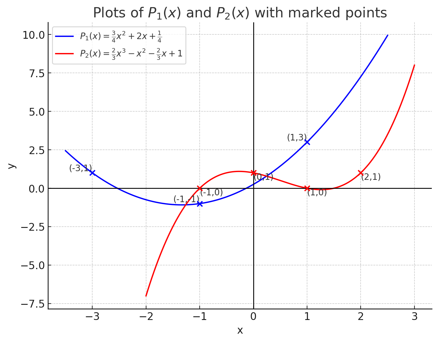
Polynomial Representation
Coefficient Representation
To illustrate this representation visually,we can use an interactive graph where the coefficients can be adjusted:
Value Representation
A polynomial can also be uniquely defined by its values at some specific points. For example, two points define a unique line:
- For points and , we have .
- For points and , we have .
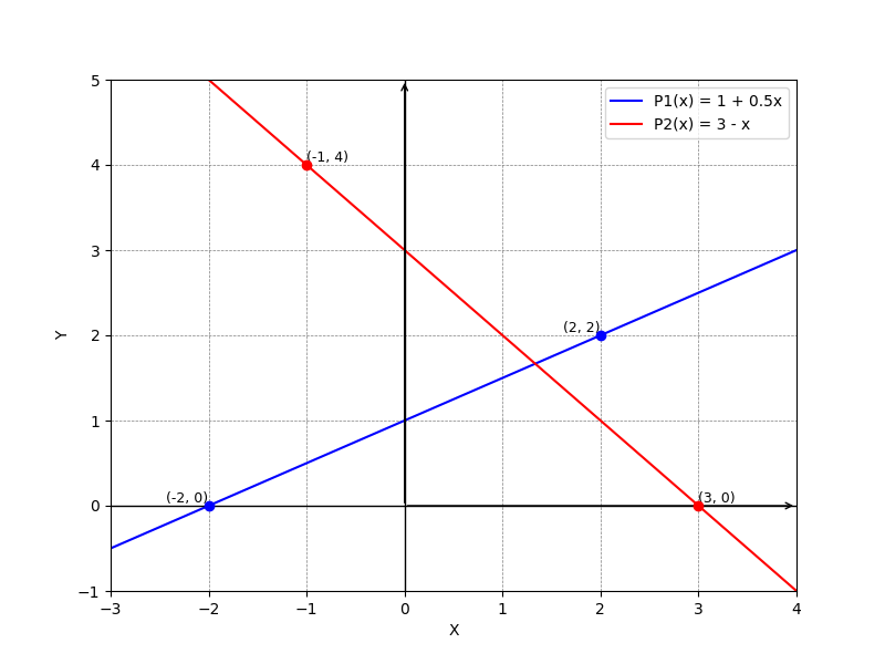
Three points define a quadratic polynomial:
More generally, points uniquely define a polynomial of degree : That is: is invertible for unique Unique exists Unique polynomial exists.
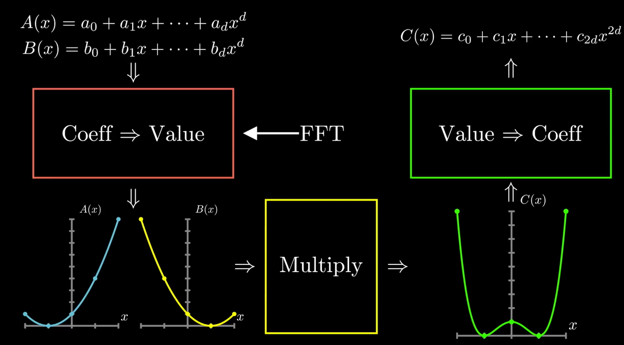
Punchline: Two Unique Trpresentations for Polynomials
Value Representation Advantages
and
In value representation, multiplication can be performed in linear time rather than quadratic . This is especially advantageous when working with large polynomials.
Polynomial Multiplication Flowchart
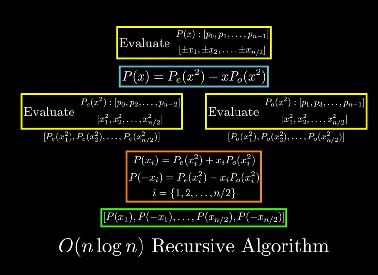
Polynomial Evaluation
Evaluation from Coefficients to Values
To evaluate a polynomial at points,we can compute as follows: Howerer, this operation can have a complexity of , which could lead to .
More Efficient Strategies
For example, when evaluatiing at 8 points, we can select symmetric points such as
.
We have .
For we can select:
We have .
So we only need 4 points!
But that is one major problem.
 We can choose the roots of unity in the finite field.
Which Evaluation Points to Use?
To evaluation , we need at least points, ideally for . The points chosen should be the roots of unity:
whers is a root of .
NTT Implementation
def FFT(P):
    # P- [p0,p1,...,p_{n-1}] coeff representation
    n=len(P) # n is a power of 2
    if n==1:
        return P
    w = get_root_of_unity(n)
    P_e,P_o = [P[0],P[2],...,P[n-2]],[P[1],P[3],...,P[n-1]]
    y_e,y_o = FFT(P_e), FFT(P_o)
    y = [0]*n
    for j in range(n/2):
        y[j] = y_e[j]+w^j*y_o[j]
        y[j+n/2] = y_e[j]-w^j*y_o[j]
    return y
Interpolation and Inverse NTT
Alternative Perspective on Evaluation/NTT
That is
Interpolation involves inversing the DFT matrix
The inverse matrix and original matrix look quite similar!
Every in original matrix is now
So the implementation of inverse NTT as follows:
def IFFT(P):
    # P- [p0,p1,...,p_{n-1}] coeff representation
    n=len(P) # n is a power of 2
    if n==1:
        return P
    w = 1/n*(get_root_of_unity(n)^{-1})
    P_e,P_o = [P[0],P[2],...,P[n-2]],[P[1],P[3],...,P[n-1]]
    y_e,y_o = FFT(P_e), FFT(P_o)
    y = [0]*n
    for j in range(n/2):
        y[j] = y_e[j]+w^j*y_o[j]
        y[j+n/2] = y_e[j]-w^j*y_o[j]
    return y
Multi-Scalar Multiplication
The Multi-Scalar Multiplication(MSM) problem involves calculating the sum of multiple elliptic curve points, represented ad:
Here, are scalars(integers modulo a prime), are elliptic curve points. indicates that is added to itself times.
Given that about 75% of the time spent producing a zk-SNARK proof is dedicated to , optimizing this operation is essential for enhancing overall performance.
Bucket method
We can break down the Multi-Scalar Multiplication problem into smaller sums and reduce the number of operations by applying the windowing technique. Before we compute ,it's important to note that each scalar can be represented in binary. This representation allows us to express in a more efficient manner.
For each , we can segment its binary representation into windows of size :
Using this approach, we can express the scalar multiplication as:
This allows us to rewrite the MSM problem as:
By changing the order of summation, we have:
weher we first break the scalars into windows and then aggregate the points in each window. Now we can focus on efficiently calculating each
with the inner summation over considering only points with the coefficient . This leads us to organize points into the corresponding lambda buckets(if ):
We can compute this with minimal point additions using partial sums:
Each of these operations involves just one elliptic point addition. We can obtain the final result by summing these partial sums:
Elliptic Curve And It's Applications
- Introduction
- What is Elliptic Curve
- Elliptic Curve's Applications
- Short Weierstrass curves and their representations for fast computations
Introduction
Elliptic curves are a fascinating area of mathematics with profound implications in number theory and cryptography. They provide a rich structure that can be utilized in various applications, particularly in secure communication protocols. In this article, we will explore the fundamental properties of elliptic curves, their group law, and how these mathematical concepts form the basis for several cryptographic algorithms. By understanding elliptic curves, we can gain insight into the underlying principles that ensure the security and efficiency of modern cryptographic systems.
What is Elliptic Curve
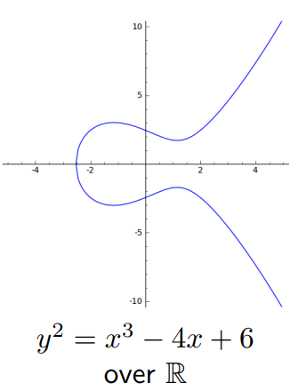
An elliptic curve is the graph of an short Weierstrass equation
where and are constants. Below is an example of such a curve.
The Group Law
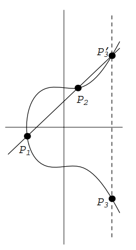
- Adding Points on an Elliptic Curve
Start with two points
on an elliptic curve given by the equation . Define a new point as follows. Draw the line through and . We'll see below that intersects in a third point . Reflect across the axis (i.e., change the sign of the -coordinate) to obtain . We define
Examples below will show that shis is not the same as adding coordinates of the points. It might be better to denote this operation by , but we opt for the simpler notation since we will never be adding points by adding coordinates.
Assume first that and that neither point is . Draw the line through and . Its slope is
If , then is vertical. We'll treat this case later, so let's assume that . The equation of is then
To find the intersection with , substitute to get
This can be rearranged to the form
The three roots of this cubic correspond to the three points of intersection of with . Generally, solving a cubic is not easy, but in the present case we already know two of the roots, namely and , since and are points on both and . Therefore, we could factor the cubic to obtain the third value of x. But there is an easier way. If we have a cubic polynomial with roots , then
Therefore,
If we know two roots , then we can recover the third as .
In our case, we obtain
and
Now, reflect across the axis to obtain the point :
In the case that but , the line through and is a vertical line, which therefore intersects E in . REflecting across the axis yields the same point (this is why we put at both the top and the bottom of the axis).Therefore, in this case .
Now consider the case where When two points on a curve are very close to each other, the line through them approximates a tangent line. Therefore, when the two points coincide, we take the line through them to be the tangent line. Implicit differentiation allows us to find the slope of :
If then the line is vertical and we set , as before. Therefore, assume that . The equation of is
as before. We obtain the cubic equation
This time, we know only one root, namely , but it is a double root since is tangent to at . Therefore, proceeding as before, we obtain
Finally, suppose . The line through and is a vertical line that intersects in the point that is the reflection of across the axis. When we reflect across the axis to get , we are back at . Therefore
for all points on . Of course, we extend this to include .
Let's summarize the above discussion:
Let be an elliptic curve defined by . let and be points on with . Define as follows:
- If , then where .
- If but , then .
- If and , then , where .
- If and , then .
Moreover, define
for all points on .
The addition of points on an elliptic curve satisfies the following properties:
- (Commutativity) for all on .
- (existence of identity) for all points on .
- (existence of inverses) Given on , there exists on with . This point will usually be denoted .
- (associativity) for all on . In other words, the points on form an additive abelian group with as the identity element.
In cryptography, work over instead of . We writh group operation additively . Fix a generator of primer order . In practice, chosen from some standard(e.g. NIST).
Elliptic Curve's Applications
What is discrete logarithm problem
screct , public , recovering from is hard.
ECDSA
Elliptic Curve Digital Signature Algorithm
Diffie-Hellman Key Exchange
Schnorr protocol
wants to convince that knows a secret s.t. .
Short Weierstrass curves and their representations for fast computations
http://www.hyperelliptic.org/EFD/g1p/auto-shortw.html
Pairing based cryptography
Defination of Pairing
Given cyclic groups all same prime order , a is a nondegenerate bilinera map , are the generators of ,respectively.
- Bilinearity: and
- Non-degeneracy: is a generator.
- Computability: There exists an efficient algorithm to compute .
An application: BLS signature scheme
- Keygen:
- private key: x, and Public key
- Sign(x,m): ,, where is a cryptographic hash that maps the message space to .
- Verify(): check
BLS signature scheme can be extended to allow signature aggregation.
Commitments Schemes in Cryptography
Commitment schemes are fundamental cryptographic protocols that allow one party(the committer) to commit to a value while keeping it hidden from another party(the receiver) until the commitment is revealed. These schemes provide a way for the committer to ensure that the value cannot be altered after it has been committed, thus ensuring both secrecy and integrity.
Key properties
- Hiding: The commitment should not reveal any information about the committed value. This means that the receiver cannot determine the value until the committer decides to reveal it.
- Binding: Once the committer has made a commitment, they cannot change the committed value. This encures that the committer cannot later claim to have committed to a different value.
These properties make commitment schemes useful in various cryptographic applications, including secure voting, digital signatures, and zero-knowledge proofs.
Applications
-
Secure Voting: Voters can commit to their votes and later reveal them, ensuring privacy and preventing vote manipulation.
-
Digital Signatures: Commitment schemes are often used in the generation of digital signatures, where a message is committed to before being signed.
-
Zero-Knowledge Proofs: They play a critical role in zero-knowledge proofs, where one party can prove knowledge of a value without revealing the value itself.
Polynomial commitment scheme
- Polynomial commitment schemes[KZG,10]
- Opening many polynomials at
- open a polynomial at points
- KZG Ceremony
Polynomial commitment schemes[KZG,10]
Bilinear Group: Univariate polynomials
:
- Sample random
- delete !! (trusted setup)
Honest prover:
:
- , as is a root of
- Compute and , using gp
:
check
Opening many polynomials at
Input: .
Verifier has commitments to 's wants to verifier correctness of 's.
Naive solution
Run KZG for each . Cost: group elemets in proof, pairings for verifier.
Batched opening
- Verifier sends random
- Prover computes combination
- Verifier computes commitment to as
- Prover and verifier use KZG to verify for
Cost: verifier scalar muls to compute
open a polynomial at points
thm[BDFG]: We can open a polynomial at points with 2 verifier scalar mults no matter how large is.
KZG Ceremony
A distributed generation of s.t. no one can reconstruct the trapdoor if at least one of the participants is honest and discards their secrets.
- Sample random , update with secret !
- Check the correctness of
- The contributor knows s.t.
- consists of consecutive powers and
Introductin of ZKP
What is a Zero Knowledge Proofs?
Zero-knowledge proofs (ZKPs) allow me to prove that I know a fact without revealing the fact itself. For example:
- I know the private key corresponding to an Ethereum account, but I won't disclose what that key is!
- I know a number such that SHA256(x)=0xa4865c2cae9713e9bcea7810ae83b14d18cfc259926cac793bf0ac7752851e8c ,but I won't reveal x!
In Ethereum, all transactions are secured using digital signatures based on public-key cryptography. Each public account is linked to a secret private key, and you cannot send funds from an account unless you possess that private key. A signature attached to every transaction essentially acts as a zero-knowledge proof that you know the corresponding private key. Although ZKPs might seem new, digital signature schemes have existed for decades.
Three properties of ZK Protocols
- [Zero Knowledge] The Prover's responses do not disclose the underlying information.
- [Completeness] If the Prover knows the underlying information, they can always respond satisfactorily.
- [Soundness] If the Prover doesn't know the underlying information, they'll eventually get caught.
What are zkSNARKs?
zkSNARKs are a modern cryptographic tool that enables the efficient generation of a zero-knowledge protocol for any problem or function. Their properties include:
- zk: Hides inputs
- Succinct: Generates short proofs that can be verified quickly
- Noninteractive: doesn't require a back-and-forth communication
- ARgument of Knowledge: provers you know the input
Overview of ZKP Generation
- Transform your problem (e.g., graph isomorphism, discrete logarithm) into a function whose inputs you wish to conceal.
- Convert that function into an equivalent set of "R1CS"(Rank-1 Constraint System, or other) equations:
- This is essentially an arithmetic circuit composed of "+" and "*" operations on prime field elements.
- Simplified, the equations take the form , or .
- Generate a ZKP for satisfiability of the R1CS.
Types of SNARKs
There are two main types of SNARKs:
- Short Proofs with Higher Proving Time ComplexityThese SNARKs offer compact proofs but have a prover time complexity of . Examples include Groth16 and Plonk-KZG.
- Longer Proofs with Faster Proving Times These SNARKs prioritize faster proving times, resulting in longer proofs. Examples include FRI-based proofs, also known as STARKs (e.g., Plonky2).
The PLONK IOP for general circuits
PLONK: a poly-IOP for a general circuit
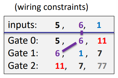
Step 1: compile circuit to a computation trace (gate fan-in=2)

The computation trace (arithmetization):
| left inputs: | right inputs: | w | |
|---|---|---|---|
| inputs: | 5 | 6 | 1 |
| Gate 0: | 5 | 6 | 11 |
| Gate 1: | 6 | 1 | 7 |
| Gate 2: | 11 | 7 | 77 |
Encoding the trace as a polynomial
Notion:
,
let (in example, ) and
The plan:
prover interpolates a polynomial that encodes the entire trace.
Prover interpolates such that
(1) encodes all inputs: for
(2) encodes all wires: :
- left input to gate #
- right input to gate #
- output of gate #
In the example, Prover interpolates such that:
| inputs: | |||
|---|---|---|---|
| Gate 0: | |||
| Gate 1: | |||
| Gate 2: |
degree() = 11
Prover can use IFFT to compute coefficients of in time
Step 2: proving validity of
Prover needs to prove that is a correct computation trace:
(1) encodes the correct inputs,
(2) every gate is evaluated correctly,
(3) the wiring is implemented correctly,
(4) the output of last gate is 0
Proving (4) is easy: prove
Proving (1): T encodes the correct inputs
Both prover and verifier interpolate a polynomial that encodes the -inputs to the circuit:
In the example: ( is linear)
constructing takes time proportional to the size of input verifier has time do this.
Let (points encoding the input)
Prover proves (1) by using a ZeroTest on to prove that
Lemma: is zero on if and only if is divisible by
Proving (2): every gate is evaluated correctly
Idea: encode gate types using a polynomial
define such that :
- if gate #l is an addition gate
- if gate #l is a multiplication gate
| inputs: | 5 | 6 | 1 | S(x) |
|---|---|---|---|---|
| Gate 0: | 5 | 6 | 11 | 1(+) |
| Gate 1: | 6 | 1 | 7 | 1(+) |
| Gate 2: | 11 | 7 | 77 | 0(\times) |
Then :
Prover uses ZeroTest to prove that for all :
Proving (3): the wiring is correct
encode the wires of :
Define a polynomial that implements a rotation:
Lemma: wire constraints are satisfied
The complete Plonk Poly-IOP (and SNARK)
Prover proves:
gates: (1)
inputs: (2)
wires: (3)
output: (4)
The eSTARK protocol is a new probabilistic proof that generalizes the STARK family through the introduction of a more generic intermediate representation called eAIR. The details can be found in estark protocol. And the prove arguments can be found in:
1. Notation
We denote by to a finite field of prime order and to its respective multiplicative group and define to be the biggest non-negative integer such that . We also write to denote a finite field extension of , of size , . Furthermore, we write (resp. ) for the ring of polynomials with coefficients over (resp. ) and write (resp. ) to denote the set of polynomials of degree lower than .
2.Multiset Equality
The details and examples can be found in Permutation argument.
Grand Product
let is a cyclic subgroup of of order n.
Given two vectors and in , a multiset equality argument, denoted , is used for checking that is equal to as multisets (or equivalently, that and are a permutation of each other). The protocol that instantiates the multiset equality arguments works by computing the following grand product polynomial : where is the value sent from the verifier.
Soundness of Multiset Equality
Lemma 1: Fix two vectors and in . If the following holds with probability larger than over a random : Then . As a consequence of Lemma 1, the identities that must be checked by the verifier for are the following:
where are the polynomials resulting from the interpolation of and over ,respectively.
The commitment polynomial is the grand product polynomial . and the two constraints is express in Eq .
3.Connection
The protocol for a connection argument and the definitions and results we provide next are adapted from GWC19. The details and examples can be found in Connection argument.
Given some vectors and a partition of the set , a connection argument, denoted , is used to check that the partition divides the field elements into sets with the same value. More specifically, if we define the sequence by:
for each , then we have if and only if belong to the same block of .
In order to express the partition within a grand product polynomial, we define a permutation as follows: is such that for each block of , σ(T ) contains a cycle going over all elements of . Then, the protocol that instantiates the connection arguments works by computing the following grand product polynomial :
where are the values sent from the verifier.
The definition of the previous polynomial is based on the following lemma, a proof of which can be found in Claim A.1. of GWC19.
Lemma 2 Fix and a partition of the set . If the following holds with probability larger than over a randoms : As a consequence of Lemma 2, the identities that must be checked by the verifier for are the following: where is the polynomial mapping G-elements to indexes in [kn] and is the polynomial defined by . For more details see GWC19.
The commitment polynomial is the grand product polynomial . and the two constraints is express in Eq .
4.inclusion
The protocol for an inclusion argument and the definitions and results we provide next is adapted from the well-known Plookup protocol GW20, with the “alternating method” provided in [PFM+22](https://eprint.iacr.org/ 2022/086). The details and examples can be found in Inclusion argument.
Given two vectors and in , a inclusion argument, denoted , is used for checking that the set A formed with the values is contained in the set B formed with the values . Notice that .
In the protocol, the prover has to construct an auxiliary vector containing every element of f and t where the order of appearance is the same as in . The main idea behind the protocol is that if , then f contributes to s with repeated elements. To check this fact, a vector is defined as follows: Then, the protocol essentially checks that is consistent with the elements of f, t and s. To do so, the vector s is split into two vectors . In the protocol described in GW20, and contain the lower and upper halves of s, while in our protocol in [PFM+22](https://eprint.iacr.org/ 2022/086), we use to store elements with odd indexes and for even indexes, that is: With this setting in mind, the grand product polynomial is defined as: where are the values sent from the verifier.
The definition of the previous polynomial is based on the following lemma, which is a slight modification of Claim 3.1. of GW20.
Lemma 3 (Soundness of Inclusion). Fix three vectors and with elements in . If the following holds with probability larger than over randoms : then and is the sorted by concatenation of and .
As a consequence of Lemma 3, the identities that must be checked by the verifier for are the following: where are the polynomials resulting from the interpolation of and over , respectively; and are the polynomials resulting from the interpolation of the values defined in Eq over .
The commitment polynomial is the grand product polynomial and and . and the two constraints is express in Eq .
5.From Vector Arguments to Simple Arguments
Let’s explain first how we reduce vector inclusions or multiset equalities to simple (i.e., involving only one polynomial on each side) inclusions or multiset equalities.
Definition 1 (Vector Arguments). Given polynomials for , a vector inclusion, denoted , is the argument in which for all there exists some such that: A vector multiset equality, denoted , is the argument in which for all there exists exactly one for which Eq holds. That is, (vector) multiset equalities define a bijective mapping.
To reduce the previous vector arguments to simple ones, we make use of a uniformly sampled element . Namely, instead of trying to generate an argument for the vector relation, we define the following polynomials: and proceed to prove the relation or . Notice that both and are in general polynomials with coefficients over the field extension even if every coefficient of , is precisely over the base field .
The previous reduction leads to the following result.
Lemma 4. Given polynomials for and as defined by Eq., if (resp. ), then (resp.) except with probability over the random choice of .
6.From Selected Vector Arguments to Simple Arguments
Now, let’s go one step further by the introduction of selectors. Informally speaking, a selected inclusion (multiset equality) is an inclusion (multiset equality) not between the specified two polynomials , , but between the polynomials generated by the multiplication of and with (generally speaking) independently generated selectors. We generalize to the vector setting.
Definition 2 (Selected Vector Arguments). We are given polynomials for . Furthermore, we are also given two polynomials whose range over the domain is {0,1}. That is, and are selectors. A selected vector inclusion, denoted , is the argument in which for all there exists some such that: where denotes the component-wise scalar multiplication between the field element and the vector .
A selected vector multiset equality, denoted . is the argument in which for all there exists exactly one for which Eq. (15) holds.
Remark 1. Note that if , then Eq. (15) is reduced to (13); if then the argument is trivial; and if either or is equal to the constant 1, then we remove the need for or respectively.
To reduce selected vector inclusion to simple ones, we proceed in two steps. First, we use the reduction shown in Eq. to reduce the inner vector of polynomials to a single one. This process outputs polynomials . Second, we make use of another uniformly sampled as follows. Namely, we define the following polynomials: and proceed to prove the relation .
Importantly, the presentation “re-ordering” in Eq. is relevant: if had been introduced in the definition of instead, then there would be situations in which we would end up having as an inclusion value and therefore the inclusion argument not being satisfied even if the selectors are correct. See Example 1 to see why this is relevant.
Example 1. Choose . We compute the following values:
| 3 | 3 | 0 | 1 | |||||
| 1 | 1 | 0 | ||||||
| 4 | 4 | 0 | 7 | |||||
| 6 | 6 | 0 | ||||||
| 1 | 1 | 0 | 5 | |||||
| 5 | 5 | 0 | ||||||
Notice how . However, if we would have instead defined , as and then we would end up having as a inclusion value, which implies that even though , and , are correct.
To reduce selected vector multiset equalities to simple ones, we follow a similar process as with selected vector inclusions. We also first use the reduction in Eq. to reduce the inner vector argument to a simple one, but then we define the following polynomials: and proceed to prove the relation . Here, we have been able to first define since we are dealing with multiset equalities instead of inclusions.
Similarly to Lemma 4, we obtain the following result. by observing that do not grow the total degree of polynomials (either from Eq. or Eq. ) over variables .
We generalize to selected vector arguments the protocols for (simple) inclusion arguments and multiset equality arguments explained in Section 2 and 4 by incorporating the reduction strategies explained in this section. Therefore, we give next the soundness bounds for these protocols.
Lemma 5. Given polynomials for and selectors , we obtain:
- Inclusion Protocol. Let and as defined by Eq.. The prover sends oracle functions for to the verifier in the first round, who responds with uniformly sampled . Enlarge the set of identities that must be checked by the verifier in the inclusion protocol of Section 4 with:
for all , i.e., the verifier checks that polynomials are valid selectors.
- Multiset Equality Protocol. Let as defined by Eq.. The prover sends oracle functions for to the verifier in the first round, who responds with uniformly sampled . Enlarge the set of identities that must be checked by the verifier in the multiset equality protocol of Section 2 with: for all .
Example 2. Say that for all the prover wants to prove that he knows some polynomials such that: Following the previous section and this section, the polynomial constraint system gets transformed to the following one, so that for all : where we notice that the only type of argument that sometimes need to be adjusted is the connection argument.
7.On the Quotient Polynomial
We obtain a single random value and define the quotient polynomial as a random linear combination of the rational functions as follows: Note that we use powers of a uniformly sampled value instead of sampling one value per constraint. Importantly, the soundness bound of this alternative version is linearly increased by the number of
constraints ℓ, so we might assume from now on that is sublinear in to ensure the security of protocols.
8. Controlling the Constraint Degree with Intermediate Polynomials
In the vanilla STARK protocol, the initial set of constraints that one attest to compute the proof over is of unbounded degree. However, when one arrives at the point after computing the quotient polynomial , it should be split into polynomials of degree lower than to ensure the same redundancy is added as with the trace column polynomials for a sound application of the FRI protocol. In this section, we explain an alternative for this process and propose the split to happen “at the beginning” and not “at the end” of the proof computation.
Therefore, we will proceed with this approach assuming that the arguments in Section 2-4 are included among the initial set of constraints. The constraints imposed by the grand products polynomials of multiset equalities and inclusions are of known degree: degree 2 for the former and degree 3 for the latter. Based on this information, we will propose a splitting procedure that allows for polynomial constraints up to degree 3 but will split any exceeding it.
Say the initial set of polynomial constraints contain a constraint of total degree greater or equal to 4. For instance, say that we have with: Now, instead of directly computing the (unbounded) quotient polynomial and then doing the split, we will follow the following process:
-
Split the constraints of degree into constraints of degree lower or equal than 3 through the introduction of one formal variable and one constraint per split.
-
Compute the rational functions . Notice the previous step restricts the degree of the ‘s to be lower than 2.
-
Compute the quotient polynomial and then split it into (at most) two polynomials and of degree lower than as follows: where is obtained by taking the first coefficients of and is obtained by taking the last coefficients (filling with zeros if necessary).
Remark 2*.* Here, we might have that is identically equal to 0. This is in contrast with the technique used for the split in Vanilla STARK, where the quotient polynomial is distributed uniformly across each of the trace quotient polynomials .
This process will “control” the degree of so that it will be always of a degree lower than 2.
Following with the example in Eq. , we rename to and introduce the formal variable and the constraint: Now, to compute the rational functions , we have to compose not only with the trace column polynomials but also with additional polynomials corresponding with the introduced variables . We will denote these polynomials as and refer to them as intermediate polynomials.
Hence, the set of constraints in gets augmented to the following set: where we include the variable in for notation simplicity. Note that now what we have is two constraints of degree lower than 3, but we have added one extra variable and constraint to take into account.
Discussing more in-depth the tradeoff generated between the two approaches, we have for one side that deg() = . Denote by the index of the where the maximum is attained. Then, the number of polynomials in the split of is equal to: which is equal to either deg() − 1 or deg().
We must compare this number with the number of additional constraints (or polynomials) added in our proposal. So, on the other side, we have that the overall number ofconstraints is: With .
We conclude that the appropriate approach should be chosen based on the minimum value between and .
Example 3. To give some concrete numbers, let us compare both approaches using the following set of constraints: In the vanilla STARK approach, we obtain . On the other side, using the early splitting technique explained before, by substituting by and by we transform the previous set of constraints into an equivalent one having all constraints of degree less or equal than 3. This reduction only introduces 2 additional constraints: Henceforth, the early splitting technique is convenient in this case, introducing 3 new polynomials instead of the 7 that proposes the vanilla STARK approach.
Plookup
definition
Plookup was described by the original authors in [GW20] as a protocol for checking whether values of a committed polynomial, over a multiplicative subgroup of a finite field , are contained in a vector that represents values of a table . More precisely, Plookup is used to check if certain evaluations of some committed polynomial are part of some row of a lookup table .
One particular use case of this primitive is: checking whether all evaluations of a polynomial , restricted to values of a multiplicative subgroup , fall in a given range . i.e., proving that, for every , we have .
Plookup’s strategy for soundness depends on a few basic mathematical concepts described below.
Notations and preliminaries
Sets and multisets
Recall that a set is a collection of distinct objects, called elements, where repetitions and order of elements are disregarded. That is, the set is the same set as .
Yet, as multisets, is not the same as . It is because multisets take into consideration all instances of an element.
Given a multiset s, we define multiplicity to be the number of all instances of an element.
So, in the multiset ; the element 3 has multiplicity 1, while 7 is of multiplicity 2 , and lastly, 1 has multiplicity 3.
A set can therefore be described as a collection of distinct objects where multiplicity and ordering of objects have no significance.
Multisets are similar to sets in that they also do not respect the ordering of elements. That is, and represent the same multiset, because they both contain the same elements, each with the same multiplicity.
Given multisets and , s can be sorted by t as follows, . That is, “ sorted by ” means the elements of are ordered according to the order they appear in , without losing their multiplicity.
Sorted multisets and set differences
Unless otherwise stated, all sorted multisets are henceforth sorted by , where is the set of natural numbers .
For any given sorted multiset , define the set of differences of s as the set of non-zero differences . That is, zero-differences, , are discarded.
Take as examples the following sorted multisets: and . These three multisets have the same set of differences, which is .
Although has the same set of differences as and , note that the differences appear in a different order; 4 appeared first then 2.
Testing for containment
Let and be ordered multisets, and none of the elements of are repeated.
It can be observed that:
-
If and , then and have the same set of differences and the differences appear in the same order.
-
If and have the same set of differences except for the differences’ order of appearance, then .
-
If and have the same set of differences and the differences appear in the same order, then .
It follows from these three observations that the criteria for testing containment boils down to checking:
- The equality of the sets of differences, and
- The order in which the differences appear in both multisets are the same.
Testing for repeated elements
Consider again the ordered multisets: and .
If has some repeated elements, for some , then these can be tested by comparing randomized sets of differences.
A randomized set of differences related to is created by selecting a random field element and defined as the set .
So, instead of a pair of repeated elements yielding a difference of zero because , they yield: in the setting of randomized set of differences.
This property of repeated elements yielding a multiple of , characterizes repeated elements in ordered multisets. Consequently, when computing randomized set of differences, repeated elements can be identified by these multiples of .
A test can therefore be coined using a grand product argument akin to the one used in PLONK’s permutation argument [GWC19].
Vectors
The above concepts defined for multisets apply similarly to vectors, and the Plookup protocol also extends readily to vectors.
A vector is a collection of ordered field elements, for some finite field , and it is denoted by .
A vector is contained in a vector , denoted by , if each for .
The vector of differences of a given vector is defined as the vector , which has one less component (or element) compared to a. That is, because .
Given a random scalar in a field F and a vector , a randomized vector of differences of is defined as .
The concatenation of vectors and is the vector , and it has n+d components.
Plookup protocol
The context of Plookup is within a polynomial commitment scheme, where a party ,called the prover, seeks to convince the second party , called the verifier, that it knows a certain polynomial.
The protocol, as described in the Plookup paper, mentions a third party called the Ideal party, denoted by , which is also called the trusted party.
It is this trusted party who is responsible for generating all the proof-verification system parameters. Among these parameters are the so-called preprocessed polynomials.
In the case of a non-interactive proof-verification system, the trusted party is equipped so as to act as an intermediary between the prover and the verifier.
-
The protocol starts with the generation of preprocessed polynomials {} and describing them as a Lookup Table.
-
Prover submits messages in the form of polynomials {} expressed either as multisets or vectors.
-
The verifier also sends randomly selected field elements , called challenges.
-
The prover then evaluates a special polynomial on the ’s and sends them to .
-
The verifier subsequently requests I to check if certain polynomial identities hold true.
-
The verifier accepts the prover’s submissions as true if all identities hold true, otherwise it rejects.
The polynomials F and G in the polynomial identities {F≡G} are bi-variate polynomials in β and γ, related to randomized sets of differences associated with {f} and {t}. They are defined in terms of grand product expressions seen below:
where and are the randomly selected field elements.
The Plookup protocol boils down to proving that the two polynomials and are the same by comparing vectors of their evaluations and multiplicities of elements in those vectors. Simply put, it checks if two polynomials are the same up to multiplicities of elements in their witness vectors.
Plookup in PIL
The test for whether the polynomial identities hold true, is based on the following lemma (viz. Claim 3.1 as stated and proved in pages 4 and 5 of the Plookup paper).
A Plookup applies to Polynomial Commitment Scheme settings, where the polynomials are expressed as vectors; , and . It is therefore a test of inclusion, denoted by .
In the zkEVM setting, Plookup typically appears in PIL code as: where in is a PIL keyword for set inclusion, .
Plookup in zkProver
The commitment of the Plookup protocol is implemented on round 2 of eSTARK. The prover computes the reducing challenges :
Using and , the prover computes the inclusion polynomials for each inclusion argument, with , and commits to them.
Connection arguments
The connection arguments is called copy-satisfy in GWC19. As its name, the argument is used to partition the commitment matrix and make the cells of the matrix in same partition contain the same value.
The Polynomial Identity Language (PIL) use **connect ** keyword to express connection arguments.
Definition
Given a vector and a partition of [n]. If for each , the whenever , and , then the elements whose indices in one are connected(copy-satisfy).
Example
Let be a specified partition of column with 6 elements. Observe the two columns depicted below:
| a | b |
|---|---|
| 3 | 3 |
| 9 | 9 |
| 3 | 7 |
| 1 | 1 |
| 3 | 3 |
| 1 | 1 |
the column a is copy-satisfy because the indices of elements in is 1, 3, 5. and ; the indices of elements in is 4, 6. and .
the column b is not copy-satisfy because the indices of elements in is 1, 3, 5. but .
Given the column a as above. we can construct a permutation map . Such for each , the map can make the elements whose indices in form a circle: 1 -> 3, 3 -> 5, 5 -> 1; 4 -> 6, 6 -> 4; 2->2.
In the zero-knowledge proof(ZKP), use the exponent of multiplicative generator() as the value of column SA of map: So in this example, the column a and the column SA as below table:
| a | SA |
|---|---|
| 3 | |
| 9 | |
| 3 | |
| 1 | |
| 3 | |
| 1 |
PIL
In the PIL context, the previous connection argument between a column a and a column SA, encoding the values of as , can be declared using the keyword connect using the syntax a connect {SA}:
the snippet of code as below:
include "config.pil";

namespace Connection(%N);
pol commit a;
pol constant SA;

{a} connect {SA};
Inclusion arguments
For most of the programs used in the zkEVM’s Prover, the values recorded in the columns of execution traces are field elements. In many cases, there may be a need to restrict the sizes of these values to only a certain number of bits. For example the variate with uint32 type, needs restricting the range from 0 to . It is therefore necessary to devise a good control strategy for handling both underflows and overflows. This document introduces the addition of 2-byte numbers as the scene using Inclusion arguments.
Verify addition of 2-byte numbers
The addition of uint16 type is a common data type in programming. It can be constrained as the below trace table:
| Row | a | b | prevCarry | Carry | Add | Reset |
|---|---|---|---|---|---|---|
| 1 | 0x11 | 0x22 | 0x01 | 0x00 | 0x33 | 1 |
| 2 | 0x30 | 0x40 | 0x00 | 0x00 | 0x70 | 0 |
| 3 | 0xff | 0xee | 0x00 | 0x01 | 0xed | 1 |
| 4 | 0x00 | 0xff | 0x01 | 0x01 | 0x00 | 0 |
The constraint is: We use as the carry in and as the carry out. becasue the lowest endian byte of uint16 not use , we use as the flag of the lowest endian byte.
The snippet of PIL code as follows:
namespace TwoByteAdd(%N);

pol constant RESET;
pol commit a, b;
pol commit carry , prevCarry , add;

prevCarry ' = carry;
a + b + (1-RESET)*prevCarry = carry*2**8 + add;
The above equation (1) only constrains the coerectness of addition, but not constrains the columns of , is 8-bits integer which range form 0 to 255. It also not constrains the columns of , , is 1-bit bool type.
An inclusion argument is used for this purpose.
Inclusion argument
Given two vectors, and , it is said that:
is contained in if such that .
In other words, if one thinks of and as multisets and reduce them to sets (by removing the multiplicity), then is contained in if is a subset of .
A protocol (,) is an inclusion argument if the protocol can be used by to prove to that one vector is contained in another vector.
In the PIL context, the implemented inclusion argument is the same as the Plookup method provided in GW20, also discussed here
An inclusion argument is invoked in PIL with the in keyword.
Specifically, given two columns and , we can declare an inclusion argument between them using the syntax: {} in {}.
Generalized inclusion arguments
In PIL we can also write inclusion arguments not only over single columns but over multiple columns. That is, given two subsets of committed columns and of some program(s) we can write as,
{} in {}
A natural application for this generalization shows that a set of columns that a program repeatedly computes, probably with the same pair of inputs/outputs. Following on with the previous “2-byte addition” program example, one can construct five new constant polynomials; BYTE_A, BYTE_B, BIT_PRECARRY,BIT_CARRY and BYTE_ADD; containing all possible byte additions.
The execution trace of these polynomials can be constructed as follows, the total number of rows is = 131072:
| row | BYTE_A | BYTE_B | BIT_PRECARRY | BIT_CARRY | BYTE_ADD |
|---|---|---|---|---|---|
| 1 | 0x00 | 0x00 | 0x0 | 0x0 | 0x00 |
| 2 | 0x00 | 0x01 | 0x0 | 0x0 | 0x01 |
| 256 | 0x00 | 0xff | 0x0 | 0x0 | 0xff |
| 257 | 0x01 | 0x00 | 0x0 | 0x0 | 0x01 |
| 258 | 0x01 | 0x01 | 0x0 | 0x0 | 0x02 |
| 65535 | 0xff | 0xfe | 0x0 | 0x1 | 0xfd |
| 65536 | 0xff | 0xff | 0x0 | 0x1 | 0xfe |
| 65537 | 0x00 | 0x00 | 0x1 | 0x0 | 0x1 |
| 65538 | 0x00 | 0x01 | 0x1 | 0x0 | 0x2 |
| 65792 | 0x00 | 0xff | 0x1 | 0x1 | 0x00 |
| 65793 | 0x01 | 0x00 | 0x1 | 0x0 | 0x02 |
| 65794 | 0x01 | 0x01 | 0x1 | 0x0 | 0x03 |
| 131071 | 0xff | 0xfe | 0x1 | 0x1 | 0xfe |
| 131072 | 0xff | 0xff | 0x1 | 0x1 | 0xff |
Recall that there is no need to enforce constraints between these polynomials since they are constant and therefore, publicly known. An inclusion argument can be utilized and thus ensure a sound description of the “2-byte addition” program. The inclusion constraint is not only ensuring that all the values are single bytes, but also that the addition is correctly computed. The input is combination of five variables : BYTE_A, BYTE_B, BIT_PRECARRY,BIT_CARRY and BYTE_ADD and it must be found in the lookup table.
In addition, recall that we only have to take into account prevCarry whenever Reset is 0. PIL is flexible enough to consider this kind of situation involving Plookups. To introduce this requirement, the inclusion check can be implemented as follows:
include "config.pil";

namespace TwoByteAdd(%N);

pol constant BYTE_A, BYTE_B, BYTE_PREVCARRY, BYTE_CARRY , BYTE_ADD;
pol constant RESET;
pol commit a, b;
pol commit carry, prevCarry, add;

prevCarry' = carry;

{a, b, (1 - RESET)*prevCarry, carry, add} in {BYTE_A, BYTE_B, BYTE_PREVCARRY, BYTE_CARRY, BYTE_ADD};
Permutation arguments
Definition
Given two vectors, and , the vectors and are permutations of each other if there exists a bijective mapping such that , where is defined by: A protocol (,) is a permutation argument if the protocol can be used by to prove to that two vectors in are a permutation of each other. Unlike inclusion arguments, the two vectors subject to a permutation argument must have the same length.
In the PIL context, the permutation argument between two columns and can be declared using the keyword is and using the syntax: {} is {}. where a and b do not necessarily need to be defined in same programs. like below snippet of permutation code:
include "config.pil";

namespace A(%N);
pol commit a, b;

{a} is {b};

namespace B(%N);
pol commit a, b;

{a} is {A.b};
A valid execution trace with the number of rows N=4, for the above example, is shown in the below table. A.a, A.b and B.a are permutations of each other.
| a | b |
|---|---|
| 8 | 2 |
| 1 | 3 |
| 2 | 8 |
| 3 | 1 |
| a | b |
|---|---|
| 3 | 6 |
| 8 | 7 |
| 1 | 8 |
| 2 | 9 |
Permutation arguments over multiple columns
Permutation arguments in PIL can be written not only over single columns but over multiple columns as well.
That is, given two subsets of committed columns and of some program(s), we can write {} in {} to denote that the rows generated by columns {} are a permutation of the rows generated by columns {}.
A natural application for this generalization is showing that a set of columns in a program is precisely a commonly known operation such as XOR, where the correct XOR operation is carried out in a distinct program (see the following example).
include "config.pil";

namespace Main(%N);
pol commit a, b, c;

{a,b,c} is {in1,in2,xor};

namespace XOR(%N);
pol constant in1, in2, xor;
However, the functionality is further extended by the introduction of selectors in the sense that one can still write a permutation argument even though it is not satisfied over the entire trace of a set of columns, but only over a subset.
Suppose that we are given the following execution traces:
Notice that columns {,,} of the program A and columns {,,} of the program B are permutations of each other only over a subset of the trace.
To still achieve a valid permutation argument over such columns, we have introduced a committed column set to 1 in rows where a permutation argument is enforced, and is 0 elsewhere.
Therefore, the permutation argument is valid only if,
- is correctly computed, and
- the subset of rows chosen by in both programs shows a permutation.
The corresponding PIL code of the previous programs can now be written as follows:
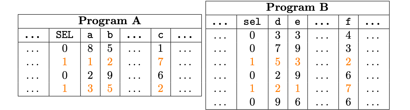
namespace A(4);
pol commit a, b, c;
pol commit sel;

sel {a, b, c} is B.sel {B.e, B.d, B.f};

namespace B(6);
pol commit d, e, f;
pol commit sel;
The column should be turned on (i.e., set to 1) the same number of times in both programs. Otherwise, a permutation cannot exist between any of the columns, since the resulting vectors would be of different lengths. This allows the use of this kind of argument even if both execution traces do not contain the same amount of rows.
fflonk
- fflonk central idea: reduce opening many polys to one using the FFT ideneity
- Cheaply opening a poly at points
Reduce opening many polys at to opening one poly at many points, then can use BDFG.
fflonk central idea: reduce opening many polys to one using the FFT ideneity
polys
First attempt: Only open the sum - . Prove that .
Problem: Doesn't constrain individually - for any will also verify
Solution: Use "FFT equation in reverse direction":
To commit to send
Assume . To open open at : i.e. give two independent constraints on !
- Similar construction can open polys at any
- Important: poly-iop based snarks work fine with a PCS that only open 'th powers.
Cheaply opening a poly at points
Notation: Given poly with commitment , , suppose for .
- Define poly of degree with for .
- Define . Then we have
- Let .Prover sends .
- From [KZG]: Verifier can now check
This requires and verifier scalar muls!
In[BDFG] we trade these scalar mults for an extra group element in the proof:
- Verifier chooses random and sends to prover.
- Define the polynomial
- If evals are correct, should be zero at
- Verifer can compute with only two scalar muls:
- Prover and verifier can now use KZG to check